letterstonature
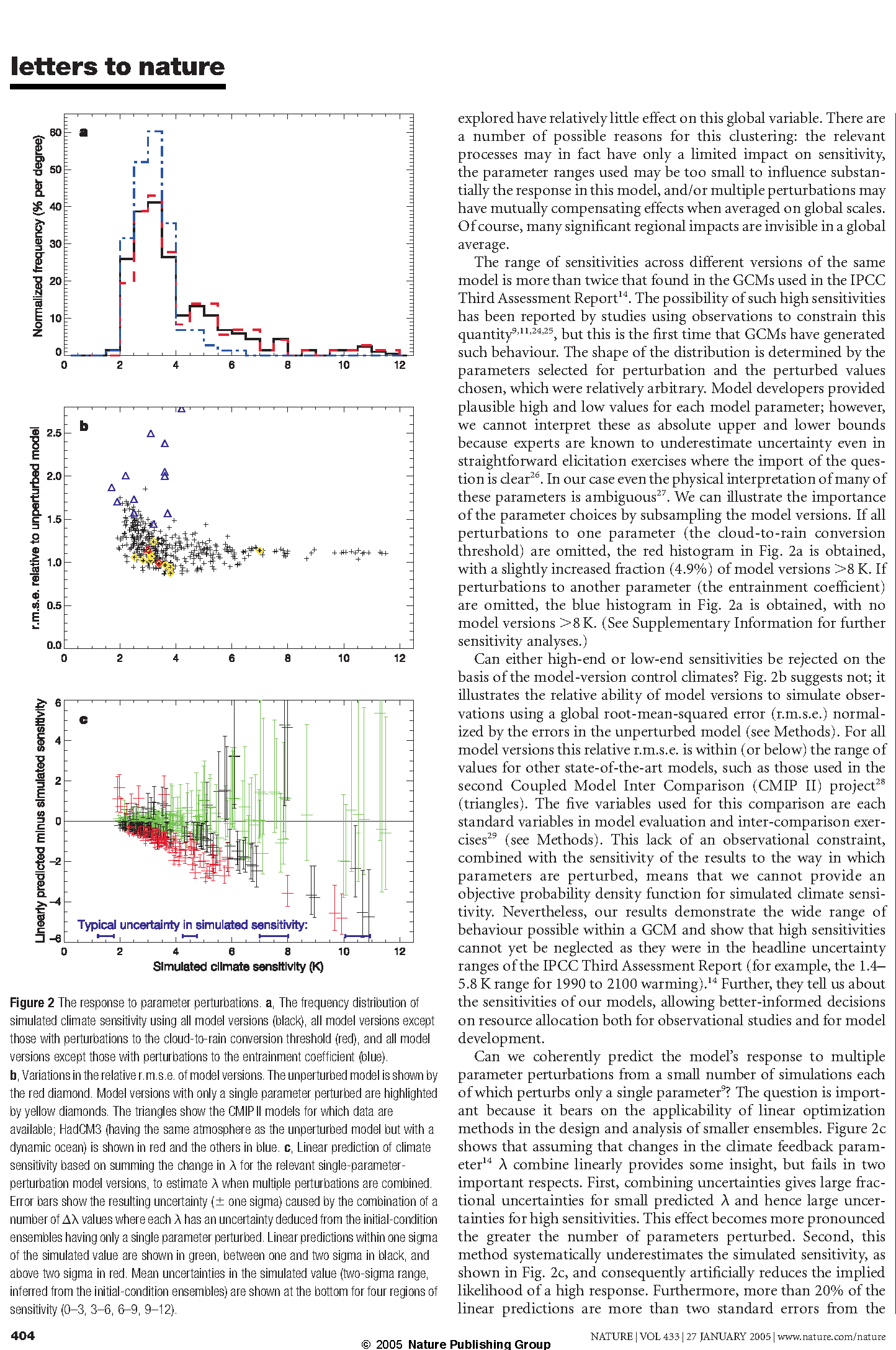
simulated sensitivities. Thus, comprehensive multiple-perturbed-parameter ensembles appear to be necessary for robust probabilistic analyses.
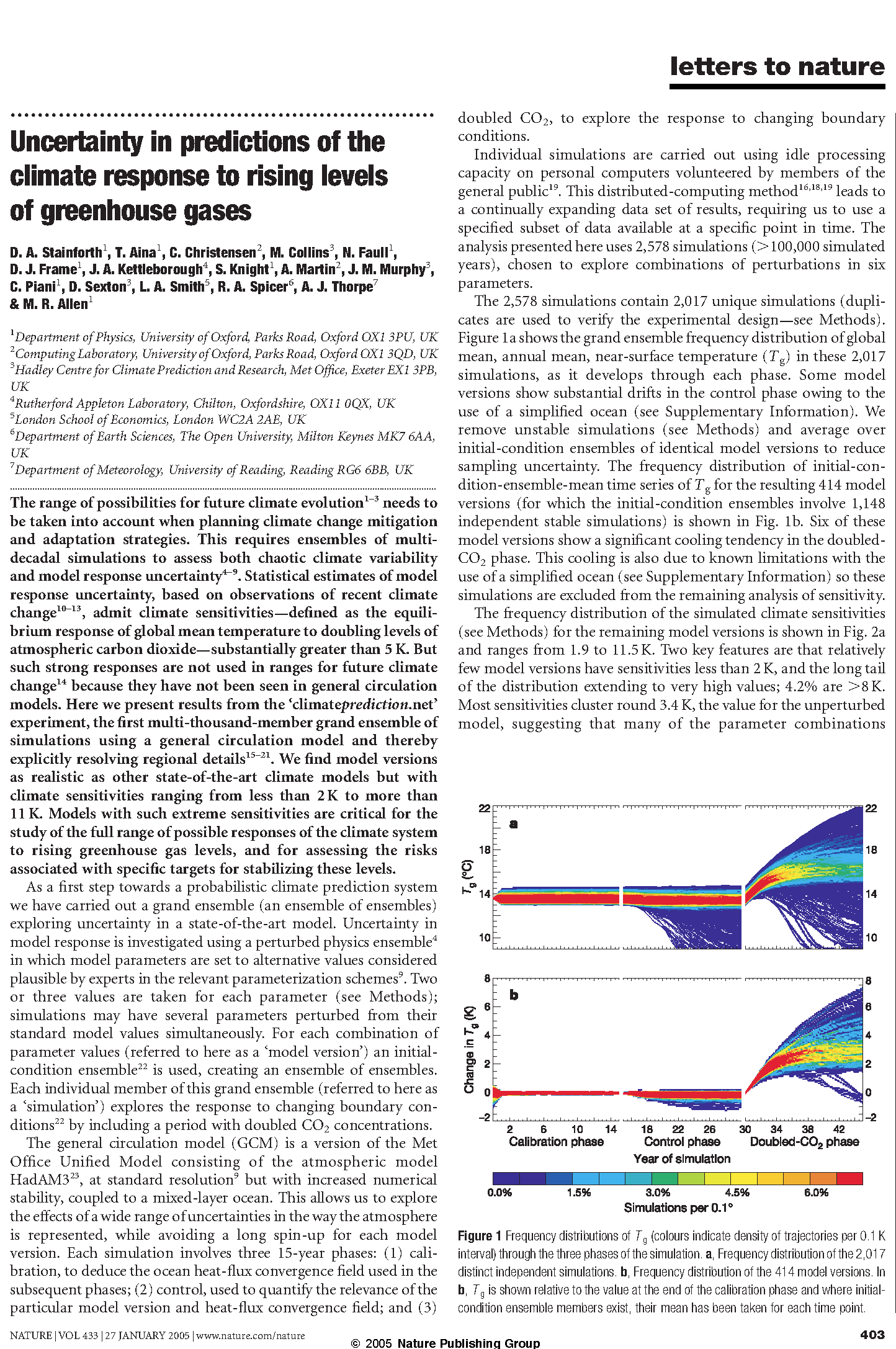
Figure 3 shows the initial-condition ensemble-mean of the temperature and precipitation changes for years 8–15 after doubling CO2 concentrations, for three model versions: (1) the unperturbed model; (2) a version with low sensitivity; and (3) a version with high sensitivity (see Supplementary Information for details of the control climates in these model versions). All three models show the familiar increased warming at high latitudes and the overall surface-temperature pattern scales with sensitivity. Even in the low-sensitivity model version the warming in certain regions is substantial, exceeding 3 K in Amazonia and 4 K in much of North America. The precipitation field shows a greater variety of response. For instance, this particular low-sensitivity model version shows a region of substantially reduced precipitation east of the Mediterranean; something not evident in either the standard or highsensitivity model versions shown. It is critical to note that model versions with similar sensitivities often also show differences in such regional details9. The use of a GCM-based grand ensemble allows the significance of such details to be ascertained.
Thanks to the participation and enthusiasm of tens of thousands of individuals world-wide we have been able to discover GCM versions with comparatively realistic control climates and with sensitivities covering a much wider range than has ever been seen before. These results are a critical step towards a better under-
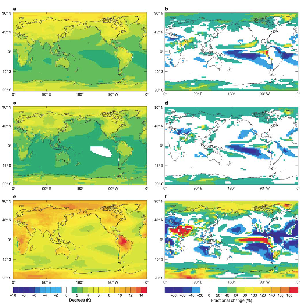
Figure 3 Thetemperature(leftpanels)andprecipitation(rightpanels)anomalyfieldsin(2.5K).e,f,Amodelversionwithhighsimulatedclimatesensitivity(10.5K).ThesefieldsresponsetodoublingtheCO2concentrations.a,b,Theunperturbedmodel(simulatedarethemeansofyearseighttofifteenafterthechangeofforcingisapplied,averagedoverclimatesensitivity,3.4K).c,d,Amodelversionwithlowsimulatedclimatesensitivityinitial-conditionensemblemembers;theyarenottheequilibriumresponse.
NATURE | VOL 433 | 27 JANUARY 2005 | www.nature.com/nature
© 2005Nature Publishing Group
letterstonature
standing of the potential responses to increasing levels of greenhouse gases, regional and seasonal impacts, our models and internal variability. Future experiments will include a grand ensemble of transient simulations of the years 1950–2100 using a model with a fully dynamic ocean. A
Methods Model simulations
Participants in the climateprediction.net experiment download an executable version of a full GCM. They are allocated a particular set of parameter perturbations and initial conditions enabling them to run one simulation: that is, one member of the grand ensemble. Their personal computer then carries out 45 years of simulation and returns results to the project’s servers. Over 90,000 participants from more than 140 countries have registered to date. The model, based on HadSM330, is a climate resolution version of the Met Office Unified Model with the usual horizontal grid of 3.758 longitude £ 2.58 latitude and 19 layers in the vertical. The ocean consists of a single thermodynamic layer with ocean heat transport prescribed using a heat-flux convergence field that varies with position and season but has no inter-annual variability. For each simulation the heat-flux convergence field is calculated in the calibration phase where sea surface temperatures (SSTs) are fixed; in subsequent phases the SSTs vary according to changes in the atmosphere–ocean heat flux. The initial-condition ensemble members have different starting conditions for the calibration and therefore allow for uncertainty in the heat-flux convergence fields used in the control and doubled-CO2 phases.
Data quality
Most model simulations are unique members of the grand ensemble, each being a combination of perturbed model parameters and perturbed initial conditions. To evaluate the reliability of the experimental design a certain number of identical simulations are distributed; most give identical results. Where they do not, they are usually very similar, suggesting that a few computational bits were lost at some point and consequently they are essentially different members of the initial-condition ensemble. In these cases the mean of the simulations is taken.
There are a small number of simulations (1.6%) which show obvious flaws in the data: for example, sudden jumps of data values from of the order of 102 to of the order of 108. These probably result from loss of information, for instance during a PC shut-down at a critical point in processing or a result of machine ‘overclocking’. These are removed from this analysis. Finally, runs that show a drift in T g greater than 0.02 K yr 21 in the last eight years of the control are judged to be unstable and are also removed from this analysis.
Perturbations
Perturbations are made to six parameters, chosen to affect the representation of clouds and precipitation: the threshold of relative humidity for cloud formation, the cloud-to-rain conversion threshold, the cloud-to-rain conversion rate, the ice fall speed, the cloud fraction at saturation and the convection entrainment rate coefficient. This is a subset of those explored by ref. 9. In each model version each parameter takes one of three values (the same values as those used by ref. 9); for cloud fraction at saturation only the standard and intermediate values are used. As climateprediction.net continues, the experiment is exploring 21 parameters covering a wider range of processes and values.
Climate sensitivity calculations
The simulated climate sensitivity is taken as the difference between the predicted equilibrium T g in the doubled-CO2 and control phases. The latter is simply the mean of the last eight years of that phase. The former is deduced by fitting the change in T g, relative to the start of the phase, to the exponential expression: DT g(t) ¼DT g(2£CO2)(1 2 exp(2t/t)), giving us a value of T g(2£CO2) that allows for uncertainty in the response timescale, t. Even for high simulated climate sensitivities the uncertainty in this procedure is small (see Fig. 2c) and alternative methods give similar results. Because it is based on the first 15 years’ response, the lassociated with this simulated climate sensitivity reflects the decadal timescale feedbacks in the system. Longer, centennial-timescale processes could affect the ultimate value of the equilibrium sensitivity and are best studied using models with dynamic oceans and cryospheres.
Relative root-mean-square error
Models are compared with gridded observations of annual mean temperature, sea level pressure, precipitation and atmosphere–ocean sensible and latent heat flux. The total error in variable j is defined simply as:
121s ¼ðSiwi ðmis 2 oi Þ2 ðÞ where mis is the simulated value in grid-box i averaged over the last 8 yr of the control phase of simulation s, oi is the observed value9 and wi is an area weighting. Mean squared errors relative to the standard model are computed as:
j
=N 2
1s2 ¼ðSj 1j2s =1j2u
Þ ðÞ
2
where N is the number of variables and 1j2u is the mean 1js for the unperturbed model, and averaged across initial-condition ensembles. Normalizing errors in individual variables by the corresponding errors in the unperturbed model ensures that all variables are given equal weight. The relative r.m.s.e. is plotted in Fig. 2b. Note that because we do not have an explicit and adequate noise model (1j2s does not account for correlations, for example), these ‘scores’ cannot be interpreted explicitly in terms of likelihood, but nevertheless provide an indication of the relative merits of different model control climates.
For the CMIP II data the (mi 2 oi)2 term is reduced by the variance of the mean to compensate for the greater variability found in models with dynamic oceans.
Received 4 November; accepted 20 December 2004; doi:10.1038/nature03301.
-
Schneider, S. H. What is dangerous climate change? Nature 411,17–19 (2001).
-
Reilly, J. et al. Uncertainty in climate change assessments. Science 293,430–433 (2001).
-
Wigley, T. M. L. & Raper, S. L. Interpretation of high projections for global mean warming. Science 293,451–454 (2001).
-
Allen, M. R. & Stainforth, D. A. Towards objective probabilistic climate forecasting. Nature 419,228 (2002).
-
Allen, M. R. & Ingram, W. J. Constraints on future changes in climate and the hydrological cycle. Nature 419,224–232 (2002).
-
Palmer, T. N. Predicting uncertainty in forecasts of weather and climate. Rep. Prog. Phys. 63,71–116 (2000).
-
Smith, L. What might we learn from climate forecasts? Proc. Natl Acad. Sci. USA 99,2487–2492 (2002).
-
Kennedy, M. C. & O’Hagan, A. Bayesian calibration of computer models. J. R. Stat. Soc. Ser. B Stat. Methodol. 63,425–450 (2001).
-
Murphy, J. M. et al. Quantifying uncertainties in climate change from a large ensemble of general circulation model predictions. Nature 430,768–772 (2004).
-
Knutti, R., Stocker, T. F., Joos, F. & Plattner, G. K. Constraints on radiative forcing and future climate change from observations and climate model ensembles. Nature 416,719–723 (2002).
-
Forest, C. E. et al. Quantifying uncertainties in climate system properties with the use of recent climate observations. Science 295,113–117 (2002).
-
Allen, M. R., Stott, P. A., Mitchell, J. F. B., Schnur, R. & Delworth, T. L. Quantifying the uncertainty in forecasts of anthropogenic climate change. Nature 417,617–620 (2000).
-
Stott, P. A. & Kettleborough, J. A. Origins and estimates of uncertainty in predictions of twenty-first century temperature rise. Nature 416,723–726 (2002).
-
Cubasch, U. et al. in Climate Change 2001, The Science of Climate Change (ed. Houghton, J. T.) Ch. 9 527–582 (Cambridge Univ. Press, Cambridge, 2001).
-
Allen, M. R. Do-it-yourself climate prediction. Nature 401,627 (1999).
-
Stainforth, D. et al. Distributed computing for public-interest climate modeling research. Comput. Sci. Eng. 4,82–89 (2002).
-
Hansen, J. A. et al. Casino-21: Climate simulation of the 21st century. World Res. Rev. 13,187–189 (2001).
-
Stainforth, D. et al. Climateprediction.net: Design principles for public-resource modeling. In 14th IASTED Int. Conf. on Parallel And Distributed Computing And Systems (4–6 November 2002) 32–38 (ACTA Press, Calgary, 2002).
-
Stainforth, D. et al. in Environmental Online Communication (ed. Scharl, A.) Ch. 12 (Springer, London, 2004).
-
Giorgi, F. & Francisco, R. Evaluating uncertainties in the prediction of regional climate change. Geophys. Res. Lett. 27,1295–1298 (2000).
-
Palmer, T. N. & Raisanen, J. Quantifying the risk of extreme seasonal precipitation events in a changing climate. Nature 415,512–517 (2002).
-
Collins, M. & Allen, M. R. Assessing the relative roles of initial and boundary conditions in interannual to decadal climate predictability. J. Clim. 15,3104–3109 (2002).
-
Pope, V. D., Gallani, M., Rowntree, P. R. & Stratton, R. A. The impact of new physical parameterisations in the Hadley Centre climate model – HadAM3. Clim. Dyn. 16,123–146 (2000).
-
Gregory, J. M. et al. An observationally-based estimate of the climate sensitivity. J. Clim. 15,3117–3121 (2002).
-
Andronova, N. G. & Schlesinger, M. E. Objective estimation of the probability density function for climate sensitivity. J. Geophys. Res. 106,22605–22612 (2001).
-
Morgan, M. G. & Keith, D. W. Climate-change — subjective judgments by climate experts. Environ. Sci. Technol. 29,468–476 (1995).
-
Smith, L. A. in Disentangling Uncertainty and Error: On the Predictability of Nonlinear Systems (ed. Mees, A. I.) Ch. 2 (Birkhauser, Boston, 2000).
-
Covey, C. et al. An overview of results from the coupled model intercomparison project. Glob. Planet. Change 37(1–2), 103–133 (2003).
-
McAveney, B. J. et al. in Climate Change 2001, The Science of Climate Change (ed. Houghton, J. T.) Ch. 8, 471–524 (Cambridge Univ. Press, Cambridge, 2001).
-
Williams, K. D., Senior, C. A. & Mitchell, J. F. B. Transient climate change in the Hadley centre models: the role of physical processes. J. Clim. 14,2659–2674 (2001).
Supplementary Information accompanies the paper on www.nature.com/nature.
Acknowledgements We thank all participants in the ‘climateprediction.net’ experiment and the many individuals who have given their time to make the project a reality and a success. This work was supported by the Natural Environment Research Council’s COAPEC, e-Science and fellowship programmes, the UK Department of Trade and Industry, the UK Department of the Environment, Food and Rural Affairs, and the US National Oceanic and Atmospheric Administration. We also thank Tessella Support Services plc, Research Systems Inc., Numerical Algorithms Group Ltd, Risk Management Solutions Inc. and the CMIP II modelling groups.
Competing interests statement The authors declare that they have no competing financial interests.
Correspondence and requests for materials should be addressed to D.A.S. (d.stainforth1@physics.ox.ac.uk).
© 2005Nature Publishing Group NATURE | VOL 433 | 27 JANUARY 2005 | www.nature.com/nature